Separating and uniting data

Jeff Stevens

2023-02-27

Introduction

The problem

What’s different between these data sets?

What needs to happen to create data2 from data1?

data1

# A tibble: 11 × 4
      id cond1 cond2 date      
   <int> <int> <chr> <date>    
 1     1     1 A     2022-02-06
 2     1     2 A     2022-01-17
 3     1     3 A     2022-01-27
 4     2     1 B     2022-02-28
 5     2     3 B     2022-02-15
 6     3     1 A     2022-01-20
 7     3     2 A     2022-01-11
 8     3     3 A     2022-01-30
 9     4     1 B     2022-02-26
10     4     2 B     2022-01-24
11     4     3 B     2022-01-05

data2

# A tibble: 12 × 5
      id condition year  month day  
   <int> <chr>     <chr> <chr> <chr>
 1     1 1A        2022  02    06   
 2     1 2A        2022  01    17   
 3     1 3A        2022  01    27   
 4     2 1B        2022  02    28   
 5     2 2B        <NA>  <NA>  <NA> 
 6     2 3B        2022  02    15   
 7     3 1A        2022  01    20   
 8     3 2A        2022  01    11   
 9     3 3A        2022  01    30   
10     4 1B        2022  02    26   
11     4 2B        2022  01    24   
12     4 3B        2022  01    05

Mental model of tidy data

Each variable has its own column
Each observation has its own row
Each value has its own cell

Separating data

table3

# A tibble: 6 × 3
  country      year rate             
  <chr>       <dbl> <chr>            
1 Afghanistan  1999 745/19987071     
2 Afghanistan  2000 2666/20595360    
3 Brazil       1999 37737/172006362  
4 Brazil       2000 80488/174504898  
5 China        1999 212258/1272915272
6 China        2000 213766/1280428583

Why is `table3` not tidy?

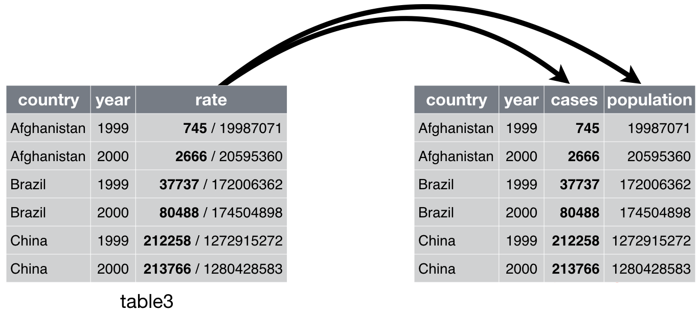
Separating data

separate(table3, rate, into = c("cases", "population"))

# A tibble: 6 × 4
  country      year cases  population
  <chr>       <dbl> <chr>  <chr>     
1 Afghanistan  1999 745    19987071  
2 Afghanistan  2000 2666   20595360  
3 Brazil       1999 37737  172006362 
4 Brazil       2000 80488  174504898 
5 China        1999 212258 1272915272
6 China        2000 213766 1280428583

separate(table3, rate, into = c("cases", "population"), convert = TRUE)

# A tibble: 6 × 4
  country      year  cases population
  <chr>       <dbl>  <int>      <int>
1 Afghanistan  1999    745   19987071
2 Afghanistan  2000   2666   20595360
3 Brazil       1999  37737  172006362
4 Brazil       2000  80488  174504898
5 China        1999 212258 1272915272
6 China        2000 213766 1280428583

Separating data

separate(table3, year, into = c("century", "year2"), sep = 2)

# A tibble: 6 × 4
  country     century year2 rate             
  <chr>       <chr>   <chr> <chr>            
1 Afghanistan 19      99    745/19987071     
2 Afghanistan 20      00    2666/20595360    
3 Brazil      19      99    37737/172006362  
4 Brazil      20      00    80488/174504898  
5 China       19      99    212258/1272915272
6 China       20      00    213766/1280428583

separate(table3, year, into = c("century", "year2"), sep = 2, remove = FALSE)

# A tibble: 6 × 5
  country      year century year2 rate             
  <chr>       <dbl> <chr>   <chr> <chr>            
1 Afghanistan  1999 19      99    745/19987071     
2 Afghanistan  2000 20      00    2666/20595360    
3 Brazil       1999 19      99    37737/172006362  
4 Brazil       2000 20      00    80488/174504898  
5 China        1999 19      99    212258/1272915272
6 China        2000 20      00    213766/1280428583

Separating data

Warning

The separate() function is being superseded by separate_wider_delim() and separate_wider_position() for the two use cases described before. But these are both listed as experimental, so we’re sticking with separate().

separate(table3, rate, into = c("cases", "population"), sep = "/")

separate_wider_delim(table3, rate, names = c("cases", "population"), delim = "/")

Separating data

Warning

separate(table3, year, into = c("century", "year2"), sep = 2)

separate_wider_position(table3, year, widths = c(century = 2, year2 = 2))

Uniting data

table5

# A tibble: 6 × 4
  country     century year  rate             
  <chr>       <chr>   <chr> <chr>            
1 Afghanistan 19      99    745/19987071     
2 Afghanistan 20      00    2666/20595360    
3 Brazil      19      99    37737/172006362  
4 Brazil      20      00    80488/174504898  
5 China       19      99    212258/1272915272
6 China       20      00    213766/1280428583

Why is `table5` not tidy?

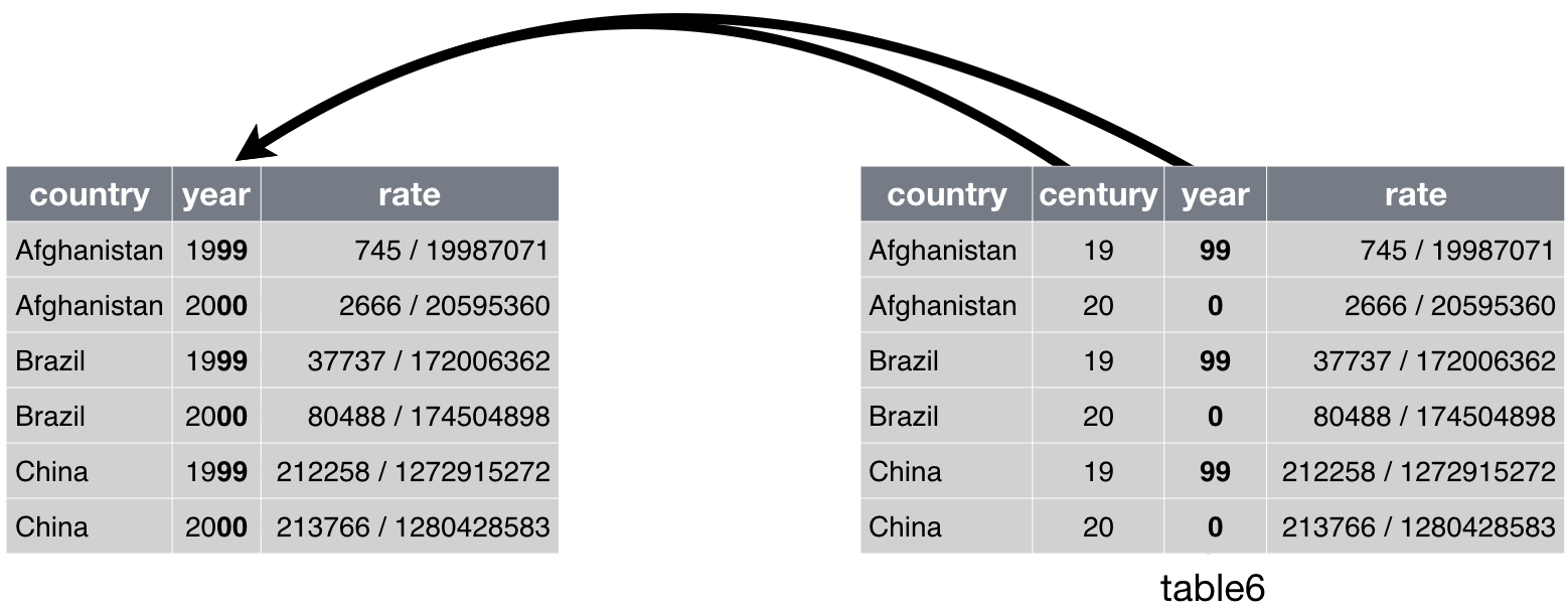
Uniting data

unite(table5, new, century:year)

# A tibble: 6 × 3
  country     new   rate             
  <chr>       <chr> <chr>            
1 Afghanistan 19_99 745/19987071     
2 Afghanistan 20_00 2666/20595360    
3 Brazil      19_99 37737/172006362  
4 Brazil      20_00 80488/174504898  
5 China       19_99 212258/1272915272
6 China       20_00 213766/1280428583

unite(table5, new, century:year, sep = "")

# A tibble: 6 × 3
  country     new   rate             
  <chr>       <chr> <chr>            
1 Afghanistan 1999  745/19987071     
2 Afghanistan 2000  2666/20595360    
3 Brazil      1999  37737/172006362  
4 Brazil      2000  80488/174504898  
5 China       1999  212258/1272915272
6 China       2000  213766/1280428583

Uniting data

unite(table5, new, century:year, sep = "", remove = FALSE)

# A tibble: 6 × 5
  country     new   century year  rate             
  <chr>       <chr> <chr>   <chr> <chr>            
1 Afghanistan 1999  19      99    745/19987071     
2 Afghanistan 2000  20      00    2666/20595360    
3 Brazil      1999  19      99    37737/172006362  
4 Brazil      2000  20      00    80488/174504898  
5 China       1999  19      99    212258/1272915272
6 China       2000  20      00    213766/1280428583

Coalescing data

coal_data

# A tibble: 4 × 3
    a_1   a_2   a_3
  <dbl> <dbl> <dbl>
1     1    NA    NA
2    NA     4    NA
3    NA    NA     7
4    NA    NA    NA

coal_data %>% # note the use of magrittr pipe!
  mutate(a_all = coalesce(!!! select(., contains("a_"))))

# A tibble: 4 × 4
    a_1   a_2   a_3 a_all
  <dbl> <dbl> <dbl> <dbl>
1     1    NA    NA     1
2    NA     4    NA     4
3    NA    NA     7     7
4    NA    NA    NA    NA

Incomplete data sets

Missing data

stocks

# A tibble: 7 × 3
   year   qtr return
  <dbl> <dbl>  <dbl>
1  2015     1   1.88
2  2015     2   0.59
3  2015     3   0.35
4  2015     4  NA   
5  2016     2   0.92
6  2016     3   0.17
7  2016     4   2.66

Explicitly missing (Q4 2015 is NA)
Implicitly missing (Q1 2016 absent)

stocks |> 
  complete(year, qtr)

# A tibble: 8 × 3
   year   qtr return
  <dbl> <dbl>  <dbl>
1  2015     1   1.88
2  2015     2   0.59
3  2015     3   0.35
4  2015     4  NA   
5  2016     1  NA   
6  2016     2   0.92
7  2016     3   0.17
8  2016     4   2.66

Important for factorial designs and for data validation

Combinations of factors

fruits

# A tibble: 6 × 4
  type    year size  weights
  <chr>  <dbl> <fct>   <dbl>
1 apple   2010 XS       1.87
2 orange  2010 S        2.64
3 apple   2012 M        5.68
4 orange  2010 S        3.70
5 orange  2010 S        4.19
6 orange  2012 M        5.83

fruits |> expand(type, size)

# A tibble: 8 × 2
  type   size 
  <chr>  <fct>
1 apple  XS   
2 apple  S    
3 apple  M    
4 apple  L    
5 orange XS   
6 orange S    
7 orange M    
8 orange L

return all possible combinations

Combinations of factors

fruits

# A tibble: 6 × 4
  type    year size  weights
  <chr>  <dbl> <fct>   <dbl>
1 apple   2010 XS       1.87
2 orange  2010 S        2.64
3 apple   2012 M        5.68
4 orange  2010 S        3.70
5 orange  2010 S        4.19
6 orange  2012 M        5.83

fruits |> expand(nesting(type, size))

# A tibble: 4 × 2
  type   size 
  <chr>  <fct>
1 apple  XS   
2 apple  M    
3 orange S    
4 orange M

return all existing combinations

Filling data

treatment

# A tibble: 4 × 3
  person           treatment response
  <chr>                <dbl>    <dbl>
1 Derrick Whitmore         1        7
2 <NA>                     2       10
3 <NA>                     3        9
4 Katherine Burke          1        4

treatment |> 
  fill(person)

# A tibble: 4 × 3
  person           treatment response
  <chr>                <dbl>    <dbl>
1 Derrick Whitmore         1        7
2 Derrick Whitmore         2       10
3 Derrick Whitmore         3        9
4 Katherine Burke          1        4

Solving the problem

What code turns data1 into data2?

data1

# A tibble: 11 × 4
      id cond1 cond2 date      
   <int> <int> <chr> <date>    
 1     1     1 A     2022-02-06
 2     1     2 A     2022-01-17
 3     1     3 A     2022-01-27
 4     2     1 B     2022-02-28
 5     2     3 B     2022-02-15
 6     3     1 A     2022-01-20
 7     3     2 A     2022-01-11
 8     3     3 A     2022-01-30
 9     4     1 B     2022-02-26
10     4     2 B     2022-01-24
11     4     3 B     2022-01-05

data2

# A tibble: 12 × 5
      id condition year  month day  
   <int> <chr>     <chr> <chr> <chr>
 1     1 1A        2022  02    06   
 2     1 2A        2022  01    17   
 3     1 3A        2022  01    27   
 4     2 1B        2022  02    28   
 5     2 2B        <NA>  <NA>  <NA> 
 6     2 3B        2022  02    15   
 7     3 1A        2022  01    20   
 8     3 2A        2022  01    11   
 9     3 3A        2022  01    30   
10     4 1B        2022  02    26   
11     4 2B        2022  01    24   
12     4 3B        2022  01    05

Let’s code!

Separating data [Rmd]

Separating and uniting data

Introduction

The problem

Mental model of tidy data

Separating data

Separating data

Why is table3 not tidy?

Separating data

Separating data

Separating data

Separating data

Uniting data

Uniting data

Why is table5 not tidy?

Uniting data

Uniting data

Coalescing data

Incomplete data sets

Missing data

Combinations of factors

Combinations of factors

Filling data

Solving the problem

Let’s code!

Why is `table3` not tidy?

Why is `table5` not tidy?